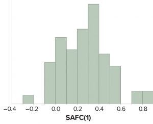
Figure 1: Values of sample autocorrelation function at lag 1 — SACF(1) — from attributes amenable to statistical analysis for continued process verification of a product line.
Control charts are used to assist in process monitoring activities. They use an estimate of central tendency (the overall mean) and variation (the standard deviation). Sample standard deviations (S) tend to underestimate process standard deviations (σ) when they are calculated using limited sample sizes of independent results (1). For this reason, the unbiasing constant c4 is used as a divisor when calculating Shewhart control-chart limits. If data used for control charting are positively autocorrelated, that tends to underestimate σ further and compromise the utility of such widely used constants.
Prevalence of Positively Autocorrelated Data in Drug Product Manufacturing
Continued process verification (CPV) is performed during stage 3 of the process validation lifecycle. The purpose of CPV is to monitor critical process parameters (CPPs), critical quality attributes (CQAs), and other attributes to demonstrate an ongoing state of control over a commercial manufacturing process.
Individuals (X chart) Shewhart control charts have been calculated and implemented for attributes amenable to statistical analyses as part of postlicensure monitoring of biopharmaceutical manufacturing processes (2). However, subject matter experts have suspected that from an early stage of commercial production, manufacturing results for specific attributes could not be considered serially independent. Consequently, estimate of the process standard deviation (σ) used in early stage control-chart limits might be underestimated, regardless of the incorporation of an unbiasing constant. Using artificially restrictive control limits can lead to an inflated type I error rate (false-positive results ) and an inappropriate dedication of resources to address such false alarms.
To assess the similarity or dissimilarity in adjacent results from manufactured lots, the sample autocorrelation function (SACF) was calculated for attributes where at least 30 batches had been dispositioned and where the data were amenable to statistical analyses. Based on the correlograms, it was noted that the lag 1 autocorrelation value was the most prominent source of internal correlation. SACF(1) results were predominantly >0, which meant that the data were positively autocorrelated.
The presence of positive autocorrelation (values closely related to each other in sequential order) can be attributed to one or more causes such as
lack of sensitivity of the analytical method
use of results with limited precision, which leads to artificially reduced variation between consecutive results
homogeneity of input factors, including raw materials.
Figure 1 shows that >75% of all CPV attributes had SACF(1) estimates between 0 and 0.5. The high percentage of SACF(1) results inside that region confirmed the suspicion that the manufacturing process could be expected to generate correlated results for many assessed CPV attributes.

Equations
Estimating Standard Deviation for Control Charts
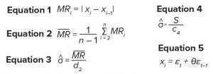
Three-sigma control limits for an X chart can be calculated using a function of the average moving range. A moving range (MR) of span 2 is calculated by taking the absolute difference of two successive observations defined in Equation 1. For a set of data containing n observations, Equation 2 can be used to calculate the average moving range. And Equation 3 can be used to calculate an estimate of σ, where d2 is an unbiasing constant determined by the span number. In the case of a moving range with span 2, d2 = ~1.128 (3). This approach to calculating control-chart limits can lead to errors when data are autocorrelated (4).
An estimate of σ also can be calculated using the sample standard deviation (S) as in Equation 4, where c4 is an unbiasing constant determined by the sample size (n). With increasing n, the value of c4 approaches 1.
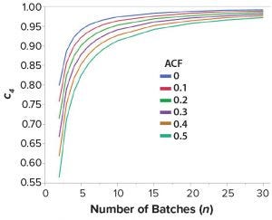
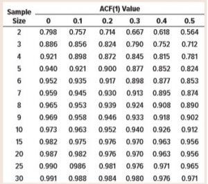
One approach to identifying more appropriate control limits when presented with autocorrelated data is to use time-series analysis. However, that may be impractical for biopharmaceutical CPV activities because of the large number of monitored attributes in bioprocessing. That is true especially for companies that manufacture multiple commercial products. Instead, the objective to “use the overall sample standard deviation for a sufficiently long, good, and stable period” has become the focus (5). For the study presented here, a series of simulations was used to calculate the values of c4 for a range of sample sizes and degree of positive autocorrelation to identify where the value of c4 is adequately close to 1 for an “expected” manufacturing experience. The values for d2 were calculated as by-products of the simulations.

Figure 2: Relationship between unbiasing constant c4 and sample size for values of ACF(1) between 0 and 0.5
Derivation of Unbiasing Constants Using Simulations
To assess the effect of both sample size and autocorrelation level on the values of c4 and d2, simulations were used based on a first-order moving average (MA) process MA(1) shown in Equation 5 (6), where t represents the time points, and θ is a nonzero constant. Values of εt were sampled randomly from a standard normal distribution. By using vast amounts of data in the simulation exercise, statistics such as SACF(1) and S approach the desired parameter values for the automated correlation function ACF(1) and σ, respectively.
Two useful aspects of the MA(1) time series for this simulation were that
We could obtain results for a predefined ACF(1) value by adjusting the value of θ.
ACF for all other lag differences are ≈0 from the simulation. The simulation strategy below can be used to calculate c4 and d2 for samples of size n = 5 with ACF(1) = 0.5:
Generate a column of data (“group”) to represent 100 million samples for n = 5.
Randomly sample 500 million values from a standard normal distribution, and represent εt.
Calculate xt using Equation 5 and θ = 1, which results in a series of data with SACF(1) of essentially 0.5, given the large dataset. Calculate the sample standard deviation using all values of x. Again, this value can be regarded as σ given the large dataset.
Calculate range and standard deviation for each group.
Calculate values of the average range and the average standard deviation from the 100 million groups of n = 5 observations.
Divide the average range and average standard deviation values from the previous step by σ to obtain d2 and c4, respectively.

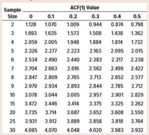
Table 1: Values of the sample moving range unbiasing constant, d2
Tables 1 and 2 list results from the simulations. Note that the values of d2 and c4 where ACF(1) = 0 match those in widely available tables used for statistical process control (SPC) activities (3). That is to be expected because the data are serially independent by design.
Practical Implications for CPV Activities
If control chart limits are to be “locked,” Figure 2 suggests that about n = 30 batches would be appropriate to estimate long-term variation across all levels of positive autocorrelation. This is because the unbiasing constant for S appears adequately close to one for ACF(1) values between 0 and 0.5. So Levey-Jennings charts (for which control limits are calculated using sample mean ±3 × S) can be used (7). That negates the requirement of including an unbiasing constant in control-chart limit calculations, once at least 30 batches of results become available.

Table 2: Values of sample standard deviation unbiasing constant, c4
Improved Process for Estimating Process Standard Deviation
Positive autocorrelation has been shown to be prevalent in manufacturing data used for monitoring biopharmaceutical products. Assuming that this is the case for other advanced biopharmaceutical manufacturing processes, use of traditional techniques to estimate σ for use in control charts may provide inappropriately narrow control limits in an X chart. Underestimating σ could increase the false-alarm rate (values exceeding a control limit), and lead to the unnecessary use of resources to “fix” a problem that does not exist. Practitioners are recommended to use Levey-Jennings control charts for fixed control-chart limits when at least 30 manufactured batches are available for analysis in CPV activities.
References
1 Zar JH. Biostatistical Analysis, 5th ed. Pearson Prentice-Hall: Upper Saddle River, NJ, 2010.
2 Montgomery DC. Introduction to Statistical Quality Control, 7th ed. Wiley Publishing: Hoboken, NJ. 2014.
3 Juran JM, Godfrey AB. Juran’s Quality Handbook, 5th Ed. McGraw-Hill: New York, NY, 1999.
4 Cryer JD, Ryan TP. The Estimation of Sigma for an X Chart: M—R/d2 or S/c4? J. Qual. Technol. 22(3) 1990: 187–192.
5 Bisgaard S, Kulahci K. Quality Quandaries: The Effect of Autocorrelation on Statistical Process Control Procedures. Qual. Eng. 17(3) 2005: 481–489.
6 Halkos G, Kevork I. Confidence Intervals in Stationary Autocorrelated Time Series. MPRA Paper 31840, University Library of Munich, Germany, 2002.
7 Levey S, Jennings ER. The Use of Control Charts in the Clinical Laboratory. Am. J. Clin. Pathol. 20(11) 1950: 1059–1066.
Keith M. Bower, MS, is senior principal CMC statistician at Seattle Genetics, Inc. and an affiliate assistant professor in the Department of Pharmacy at the University of Washington.
SAS Enterprise Guide 7.15 was used to calculate the results for Tables 1 and 2. JMP v14 software was used to generate Figures 1 and 2.
