Statistical Assessments of Bioassay Validation Acceptance Criteria

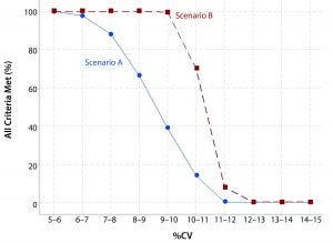
Figure 1: Likelihood meeting all criteria per scenario

Analytical linearity as well as assessments of precision and accuracy determine the range for a bioassay (1). USP <1033> recommends comparing confidence intervals (CIs) against target validation acceptance criteria in a bioassay validation exercise, but there are no clear guidelines for determining the criteria (2). Here I address several aspects of a bioassay validation, namely

CIs for the first four parameters (R², slope, intercept, and %RB) can be directly related to %CV. Doing so provides information on the likelihood of passing a set of validation acceptance criteria for a given level of bioassay precision.

Confidence Interval Calculations
To align with the bioassay validation example in USP <1033> the following assumptions are made:

Linearity is shown if the slope is equivalent to one and the intercept is equivalent to zero (there also might be a criterion on R²). CIs for the intercept and slope can be calculated using Equations 1 and 2, respectively.

Equations

Equivalence acceptance criteria (EAC) are compared with two-sided 90% CIs for the intercept and slope. If the CI is entirely contained within the interval (–EAC, EAC), then equivalence is concluded. A required minimum value for R² also can be included as validation acceptance criteria.

To assess accuracy, %RB at each level is calculated. By reexpressing the formulas in USP <1033>, lower and upper CIs for %RB are shown as Equation 3, in which SD_Ln is the standard deviation calculated using the transformed data.

Assessment of Validation Criteria
The CIs shown in Equations 1–3 and the value of R² can be related to %CV. This is achieved by considering the mean square error (MSE) from the linearity assessment as the “average” %CV across a studied range. In particular, the square root of the MSE is used in place of SD_Ln in Equation 3.

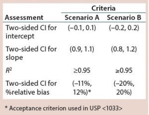
Table 1: Illustrative bioassay validation criteria

When developing a bioassay validation protocol, simulated results can provide a set of expected outcomes for predefined validation acceptance criteria in a given study design. For example, simulated data are generated using steps 1–7 in a previous article (3) and compared against two sets of validation acceptance criteria (Scenarios A and B) in Table 1.

Figure 1 shows the percentage of simulations in which all criteria for linearity and accuracy are met in relation to the calculated %CV. With stricter validation criteria, a lower frequency exists whereby all criteria are met per %CV level. Scenario A has stricter criteria than Scenario B. That is expressed most clearly once %CV exceeds around 6%. For example, if the bioassay intermediate precision %CV is expected to be 9–10%, there is about a four in 10 chance of meeting all criteria in Scenario A; however, there is essentially a 100% chance of meeting all criteria in Scenario B.

Statistical performances for acceptance criteria can be assessed using the above approach. The resulting information can guide subject matter experts in determining criteria for a bioassay validation, specific to the proposed design in the validation protocol.

References
1 <1030> Biological Assays Chapters — Overview and Glossary: IV Terms Related to Validation. USP 40–NF 35. US Pharmacopeial Convention: Rockville, MD, 2017.

2 <1033> Biological Assay Validation, Table 4. USP 40–NF 35. US Pharmacopeial Convention.

3 Bower KM. The Relationship Between R2 and Precision in Bioassay Validation in Bioassay Validation. BioProcess Int. 16(4) 2018: 26–27.

Keith M. Bower, MS, is principal CMC statistician at Seattle Genetics, Inc., 21823 30th Dr. SE, Bothell, WA 98021; 1-425-527-2104; [email protected].

SAS Enterprise Guide 7.12 software was used to generate simulated bioassay results, and Minitab v17 was used to generate the graph.