Mathematical modeling has been widely used in microbiology and biotechnology for several decades. The main objective of modeling is to find optimal conditions for microbial growth and biosynthesis of useful metabolites.

We modified the well-known equation of Perth–Marr (1) — proposed to calculate the energy consumption of a substrate— to analyze the energy consumption by cells for growth and viability maintenance. Our study includes that theory along with our own development. Our initial modeling work was carried out with Yersinia, Pseudomonas, Pasteurella, and Salmonella. For those studies, we created structured, unstructured, and general models (2, 3).

Briefly, we now propose a general model that can be described as follows. Figure 1 shows a simplified scheme of the cell cycle in prokaryotes. Positions 1 and 5 (6) correspond to the boundary points of the cell cycle — a cell of zero age. In the literature, such cells are called resting or dormant, and we call them stable cells, X^st. For bacteria, that corresponds to growth phase B, and for eukaryotic cells it is the phase of G₀ and G₁. Any intermediate position (2, 3, 4) and an infinite number of positions between them corresponds to dividing cells X^div. Such cells are most sensitive to physical, chemical, mechanical, and other influences.

Figure 1: ()

Figure 1: ()

PRODUCT FOCUS: BACTERIA-EXPRESSED PROTEINS, METABOLITES

PROCESS FOCUS: PRODUCTION, FERMENTATION

WHO SHOULD READ: PROCESS DEVELOPMENT AND MANUFACTURING

KEYWORDS: BIOMASS, CELL VIABILITY, SUBSTRATES, MATHEMATICAL MODELING

LEVEL: ADVANCED

Equation 1 is designed for calculating total biomass in our model. In that equation, n is a whole number order of the derivative of a function. Moreover, C = 1 if n = 1, and C = 0 if n ≥ 2. The factor C has the following physical sense: In growth inhibition phase (GIP), each stable cell can be divided again only one time (C_{(n = 1)} = 1). Each subsequent such transition for each separate line of cell is thus impossible (C_{(n = 2,…)} = 0). The expression is a generalized equation for any component of the biomass and for total biomass, and it unifies structured and unstructured models.

Equations 1–2

Equation 1

Equation 2

For substrates and metabolites, we suggest Equation 2, in which S (substrate) and P (target product) are substances and k^div_P,S, k^st_P,S are constants of substances rates. Therefore, biomass X with an increase in the fermentor is a “mixture” of cells of different ages. Such cells are found in all possible states, as Figure 1 shows. A versatile “mixture” consisting of different-aged cells can be characterized by parameter “age structure of populations,” which is expressed as a proportion of R cells X^st stable in the total biomass X (R = X^st/X). A higher value of R corresponds to a more complete process of fermentation.

Definitions

LGP: logarithmic growth phase

GIP: growth inhibition phase

S: substrate

X: biomass

τ: time

P: products

dP/dτ: absolute rate of product synthesis;

Q = – dS/dτ: absolute rate of substrate consumption

Q_O2: oxygen mass exchange rate, mmole O₂/(volume units per time units)

J: stochiometric factor of energy substrate (S) oxydation, Joule S/mmole O₂

µ: specific growth rate of biomass X per (hour or days)

q = Q/X or q = (1/X) × dP/dτ: a specific rate of substrate use or product synthesis

a: a trophic coefficient, amount of energy substrate consumed for the synthesis of a biomass unit

f: amount of energy substrate accumulated in biomass X during cultivation on a synthetic medium

m: an energy maintenance coefficient, the rate of substrate consumption for maintaining viability of one biomass unit per a unit of time

X_p: a maximum biomass concentration, when all the energy generated during cultivation is consumed for cell viability maintenance

X_Lim: biomass concentration in the end of exponential growth phase and beginning of growth inhibition phase

X^st: concentration of the biomass of zero age cells (stable), the content of “resting” cells

X^div: concentration of proliferation biomass

t_Lim: time of exponential growth phase termination

X_Lim^st: concentration of stable cells at the end of exponential growth phase

R: ratio of X^st to biomass X, relative content of st
able cells in the biomass, synchronization degree

X_I: initial biomass concentration in LGP corresponding the beginning of population structuring;

X_final: final biomass concentration at which R = 1 (when energy consumption is limited)

: constants of metabolite and substrate biochemical reaction rates (g of product (substrate) per g of biomass per one hour or days)

P_Lim: metabolite concentration at the end of LGP and beginning of GIP;

P₀: metabolite concentration in LGP when biomass structuring occurs at X = X_I.

Another important point is that the age structure (as revealed from our study) may change over time, not arbitrarily, but according to certain laws. Such patterns, which we have found, are the essence of the structured model that we proposed earlier for the optimization of the growth of cell populations.

It is known that stoichiometric coefficients of biochemical reactions are determined by the methods of general chemistry and biochemistry. We have accurately determined the stoichiometric coefficients of the biochemical reaction of glucose fermentation by Escherichia coli according to the structured model we proposed previously. In that case, we used experimental data from an article by Song et al (4).

Our objective for the analysis presented here is to demonstrate the possibility of describing the data obtained by Song et al. using the model shown by Klykov at al. (3, 4). We also show the possibility of determining the stoichiometric coefficients of glucose fermentation by the proposed model.

Materials and Methods

We analyzed the data for E. coli microbial culture growth, glucose consumption, and metabolites formation using the data presented by Song et al. (4) according to the model by Klykov et al. (3, 5) presented above and shown here. Briefly, a description of this model is presented by the following thesis for the slow growth phase, GIP:

Equation 3–10:

Equation 3

Equation 4

Equation 5

Equation 6

Equation 7

Equation 8

Equation 9

Equation 10

Results and Discussion

Determination of Kinetic Parameters of the Model for Biomass: In the article by Song et al. (4), Figure 6A shows anaerobic growth of E.coli glucose use as an energy substrate and biosynthesis of various metabolites. We have analyzed those processes for the proposed model of biomass growth and metabolite synthesis (3, 5). Our analysis data are presented in the following sections.

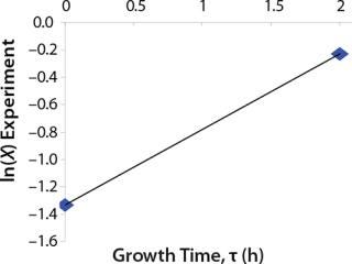
Determination of Maximum Culture Specific Growth Rate µ_max: We calculated the value of µ_max using the dependence of natural logarithm of the biomass on time, as Figure 1 and Table 1 show. For this value, the decimal logarithm log₁₀(X), — presented in Figure 6A of Song et al.(4) — was converted into a natural logarithm ln(X). Using the dependence of ln(X) on time τ, gives Equation 3. Using that equation, we calculated the coefficients µ_max and initial biomass concentration X₀ (Figures 1 and 2).

Figure 2: ()

Table 1: Initial experimental biomass and metabolite data.

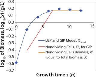
Table 1: Initial experimental biomass and metabolite data. ()

Despite the fact that the initial (exponential) growth phase is represented by only two points, it did not play a negative role for the entire analysis in general. In Klykov et al. (3), Figure 2 shows another method of determining µ_max (Table 1).

Determination of CoefficientsA,X_Lim, τ_Lim,X, and Δ⁰X (Ordinates ofFigure 4Line) Assuming X= 0: Coefficient A is calculated after the construction of dependence ΔX_2h= f(X), ΔX_2h describes biomass X concentration changes during equal time intervals Δτ= 2 h. Values ΔX_2h taken from Table 1 are presented in Figure 3. In that figure, the line crosses the x-axis at a value of X = X_p, and the y-axis at a value of X = 0 and ΔX = Δ⁰X. Figure 3 line has a slope angle equal to –0.432/h. That value represents the ratio of Δ⁰X/X_p, which is substituted into Equation 4.

Figure 3: ()

Usually, the values X_Lim and τ_Lim are determined in accordance with Figure 2 (3) and represent the points of intersection of exponential and straight lines for GIP. In our analysis, we used values corresponding to the transition (inflection) of biomass common logarithm line (Figure 1) at X = 0.76 g/L. Table 2 shows the parameters A, X_Lim, τ_Lim, and X_p as well as the parameters for the structured model. Equation 5 describes the total biomass for the logarithmic growth phase (LGP) and for the GIP.

Table 2: Biomass

Table 2: Biomass ()

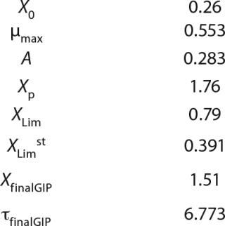
Calculation of Parameters for the Structured Model: Using Equation 6, we calculated the first parameter X^st_Lim, which represents the concentration of nondividing cells of zero age at the time of the transition from the LGP into the GIP. We then calculated the total dynamics of nondividing cells X^st for the entire process (Equation 7) using Equation 8. For further analysis, the proportion of those cells in the total biomass X — which is designated as R = X^st/X and can be calculated using Equations 9 or 10 — will be important rather than the dynamics of X^st (3).

Tables 2 and 3 show the model parameters and the calculated kinetic parameters of the biomass. Figure 2 shows that by the end of growth, the biomass — as calculated by our model at hour 6.773 — reaches stationary phase. Consequently, R amounts to 1 (Table 2 and 3) and does not change further. We then calculated the dynamics of substrate consumption and product synthesis.

Table 3: Model biomass data

Table 3: Model biomass data ()

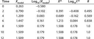
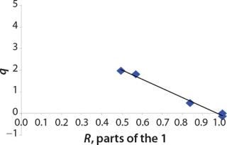
Determination of Model Parameters for Substrate Use and Metabolite Synthesis: We calculated the specific rate q substrate use and synthsis of metabolites. The parameter q for the control points (Table 3) were calculated using Equation 9. Table 4 shows the results. To calculate q, we used the values of X_τ= X_model shown Table 3 and determined in the previous step.

Table 4: Specific synthesis rates, q

Table 4: Specific synthesis rates, q ()

Calculation of the Rate Constants of Substrate Utilization and Synthesis of Metabolites,k^div: Under the proposed model of substrate utilization and synthesis of metabolites, these processes take place with different specific rates of synthesis (utilization) and degradation, k^div and k^st, which correspond to dividing cells and nondividing cells of zero age, respectively. It is assumed that any process of metabolites synthesis or substrate use may be
accompanied by the opposite process of metabolite degradation or uncontrolled reduction of substrate use rate. For example, when dividing cells are produced from a metabolite substrate, nondividing cells can in turn use it as a substrate for their biosynthesis. The kinetics of such processes, as shown previously, is well described by equations with constants k^div and k^st for different cell groups X^div and X^st.

We calcualted the constants of synthesis and utilization according to Equation 22 in an article by Klykov et al. (3), shown as Equation 10 here. Table 4 shows the values of q, and Table 3 shows the values of R. Figures (456789) are graphical representations of that equation for the metabolites and glucose taken as examples from Song et al. (4). Table 5 lists values of the constants obtained from our calcuations.

Figure 4: ()

Figure 5: ()

Figure 6: ()

Figure 7: ()

Figure 8: ()

Figure 9: ()

Table 5: Rate constants for various metabolites; relationship between these constants and the ratio between maximum concentrations of metabolites and glucose

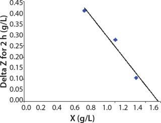
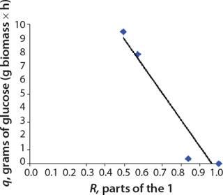
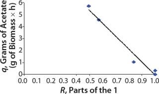
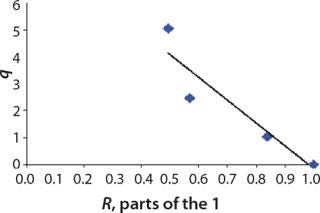
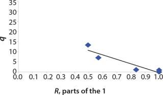
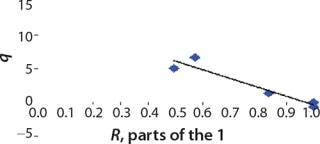
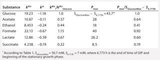
Table 5: Rate constants for various metabolites; relationship between these constants and the ratio between maximum concentrations of metabolites and glucose ()

Construction of Model Curves for the Substrate (Glucose) and Metabolites: Using the above-defined constants for the models, we designed dynamic models of glucose and metabolites according to Equations 19 and 21 in Klykov et al. (3) (Figures (101112131415).

Figure 10: ()

Figure 11: ()

Figure 12: ()

Figure 13: ()

Figure 14: ()

Figure 15: ()

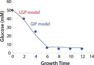
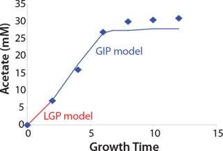
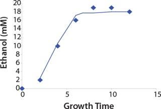
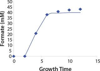
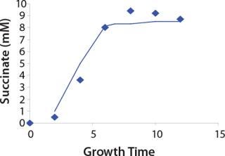
For glucose and acetate, we also calculated the process curve portions — which correspond to the exponential growth phase of the biomass (LGP). At the same time, we used constants determined from the fermentation time ranging from 2 to 6.773 hours of growth — the GIP phase. As shown in the figures, all the curves comply with experimental data, which gives evidence in favor of the proposed model.

Determination of Stoichiometric Coefficients for Glucose Fermentation According to Constants k^divand k^stfor Glucose and Metabolites:Table 5 shows the constants of metabolite synthesis and glucose utilization, k^div_i. Constants for the opposite process k^div_i in absolute value are much smaller than k^div_i, and account for only a few percents of the value k^div_i. Apparently, k^div_i = 0, and their nonzero value (Table 5) is due to the relative inaccuracy in the determination of the initial data.

Relations k^divi/k^div_Glucose are stoichiometric coefficients characterizing a quantity of metabolites produced by one mole of the used glucose. Table 5, right columns, shows the maximum values of concentrations of the produced metabolites, P_max, and their ratios to the amount of the consumed glucose, S_GlucoseMax – S6.773h. The ratios of those variables, P_max/(S_GlucoseMax – S_6.773h), are the stoichiometric coefficients, provided that k^divi = 0. That is, there are no interconversions of metabolites (not glucose) in the reactions.

As Table 5 shows, the values k^divi/k^div_Glucose and P_max/(S_GlucoseMax – S_6.773h) are practically identical. That gives evidence in favor of the assumption that k^divi = 0. That is also confirmed by the data in Table 6, which deals with the material balance for the individual atoms of carbon, hydrogen, and oxygen for biochemical reactions, described as follows:

To prepare the material balance of glucose use, we multiplied the ratios of constants k^div_i/k^div_Glucose (Table 5), as stoichiometric coefficients by the corresponding coefficients for individual chemical elements of each individual metabolite shown in Table 5. We summed the values obtained and compared those results with the corresponding values for glucose (the middle part of Table 6). As can be seen, the material balances for the chemical elements of glucose in the left side of the biochemical reaction, and the amount of metabolites in the right side of it practically coincide with the preliminary calculation.

Benefits of the Proposed Model

Our proposed structured deterministic model describes the kinetics of biomass growth. Metabolism is not worse than other models, but rather provides a simpler mathematical approach. Our model allows for analyzing the chemical stoichiometry of biological processes. Such analysis provides for the economic calculation of the industrial processes of cell culture and a real forecast of the parameters.

About the Author

Author Details
Sergey P. Klykov, PhD ([email protected]) is senior researcher, and Vladimir V. Kurakov, PhD ([email protected]) is general manager of biotechnology at PHAHARM-REGION, Ltd. 10/1, Baryshikha Street, Moscow, Russian Federation 125222; +79037951745.

REFERENCES

1.) Pirt, SJ. 1975.Principles of Microbe and Cell Cultivation, Blackwell Scientific Publications, Oxford.

2.) Derbyshev, VV. 2001. The Development Populations in Conditions of Limitation by the Energy Supply. Biotekhnologia 2:89-96.

3.) Klykov, SP. 2011. A Cell Population Structuring Model to Estimate Recombinant Strain Growth in a Closed System for Subsequent Search of the Mode to Increase Protein Accumulation During Protealysin Producer Cultivation. Biofabrication http:
//iopscience.iop.org/1758-5090/3/4/045006 3:045006.

4.) Song, H-S, and D. Ramkrishna. 2011. Cybernetic Models Based On Lumped Elementary Modes Accurately Predict Strain-Specific Metabolic Function. Biotechnol. Bioeng. 108:127-140.

5.) Klykov, SP, and VV. Derbyshev. 2009. Dependence of Cell Population Age Structure, Substrate Utilization and Metabolite Synthesis on Energy Consumption. Biotekhnologia 5:80-89.